From cell segmentation to ancient scrolls, and back again
Over the summer I worked on a Kaggle competition run by the Vesuvius Challenge, using tools designed for cell segmentation on 2000-year-old papyrus. I finished in the top 9%, 113th of 1391 teams. It was a nice opportunity to flex those image analysis skills on a different type of problem.
The Herculaneum scrolls were carbonised by Vesuvius in 79 AD and are far too fragile to unroll, so they get imaged with synchrotron CT instead. Inside each volume is a sheet of papyrus wound around itself hundreds of times (like a swiss roll!). Trace the surface of that sheet and you can flatten it out and read what’s written on it. The competition gave you a cube of CT data and asked for the centre surface of the papyrus.
A familiar problem (somewhat)!
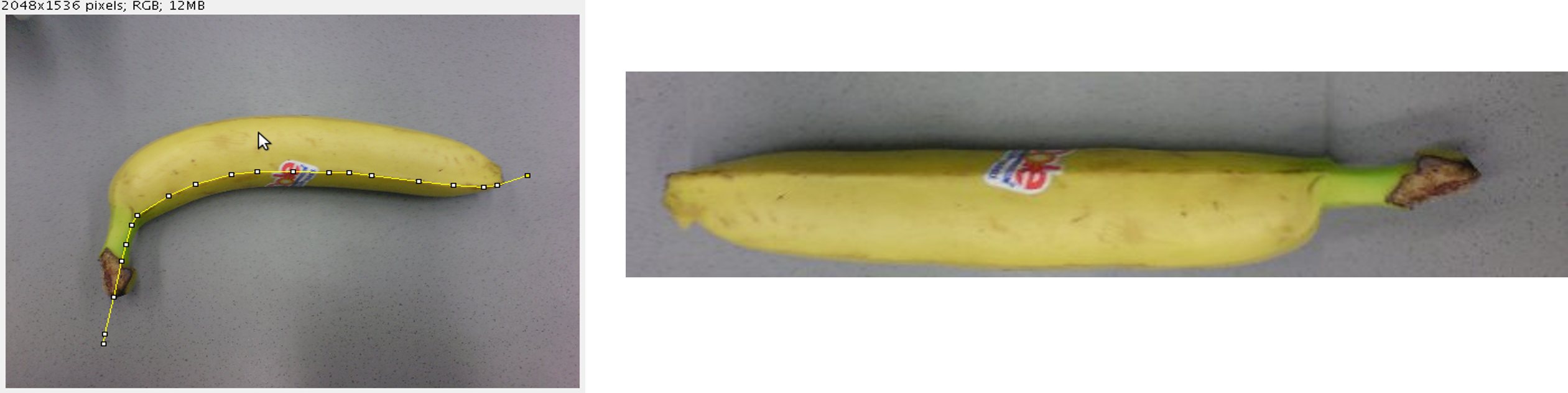
Underneath the archaeology, the task is to find thin, densely packed, self-touching sheets in noisy volumetric data. Two sheets pressed together look like one, and a sheet that is split appears like two. The signal is quite dim, and the geometry is complicated. Anyone who has segmented membranes, traced neurites or reconstructed vasculature from bioimaging data knows what I’m talking about. It reminded me of the Fiji Straighten plugin, where they show a banana for scale (literally!).
It looked straightforward at first, but you wouldn’t have a $200k prize pool if it was that simple.
So I started where I’d start with any new dataset, using familiar tools like ilastik. Paint a few labels, let the random forest do the rest.
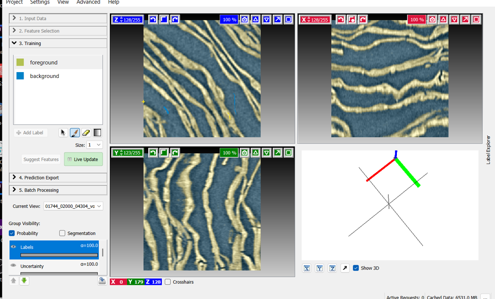
The sheet detection looked fine and contrast didn’t seem to be a problem. The bands are visible to the naked eye, and ilastik got the 3D topology largely right.
The target is not the sheet
Then I looked properly at the ground truth. To be honest it was there all along in the competition intro and on the website :)! You aren’t asked for the papyrus, but for a roughly three-voxel line through the middle of each band, where most of the written surface of that wrap sits. Segmenting the sheet gets you a thick ribbon; the competition wants the precise centre of it.
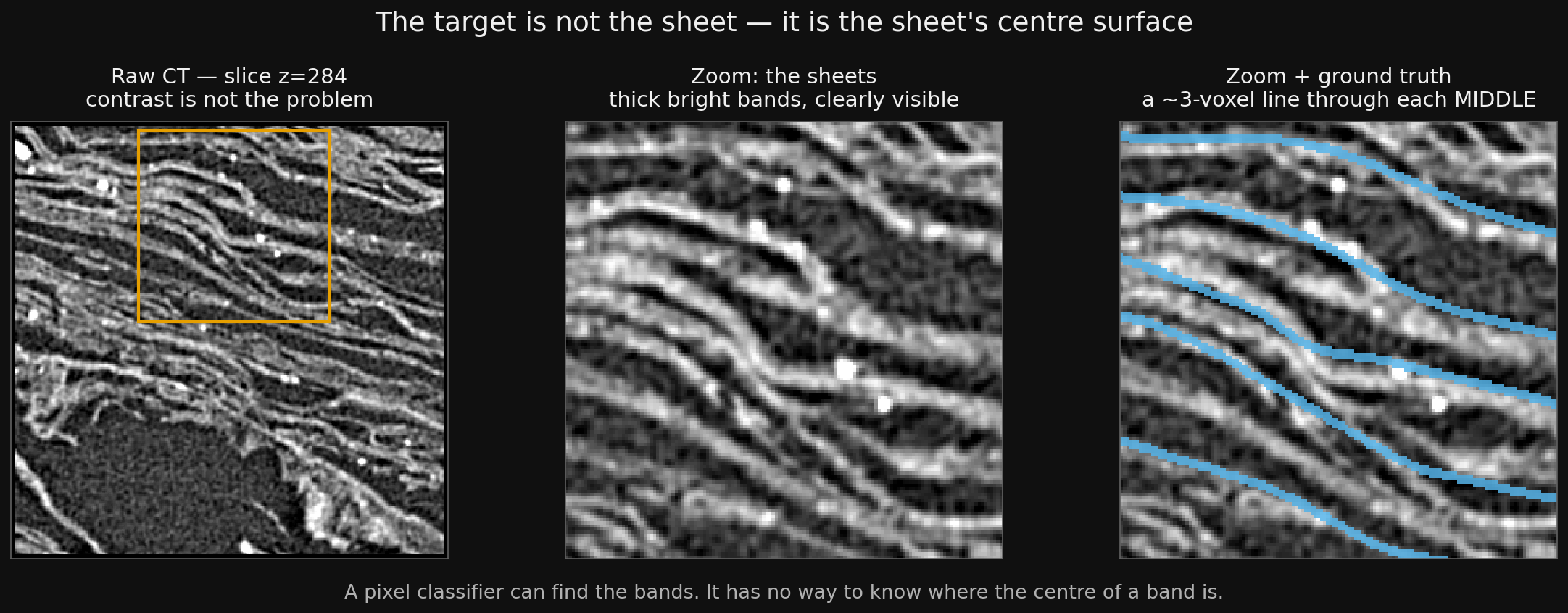
The sheets are the easy part. The target is the thin line down the middle of each one. Note how one of the blue lines goes through a split sheet
This again reminded me of how we have to predict the midline of a membrane or the centreline of a vessel, more often than not carried through a stretch where the structure is locally broken. The instruction isn’t “segment the thing” but “infer where the middle of the thing would have been.”
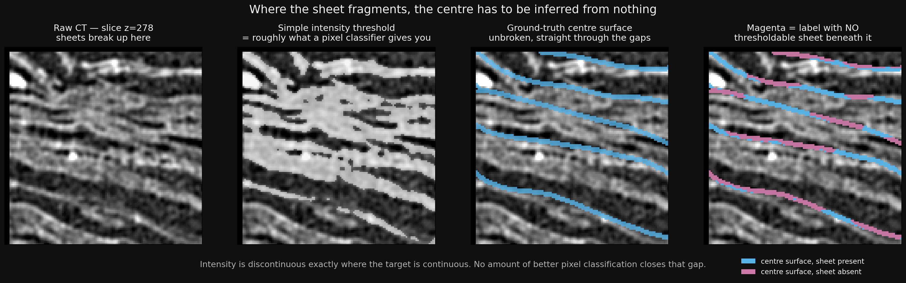
Where the sheet breaks up, the centre line has to be inferred rather than found. A threshold can’t do this.
Feeding the network a better picture
Nearly every serious team ran nnU-Net, a self-configuring segmentation framework and an extremely strong default for volumetric biomedical data. If everyone is running the same architecture, the architecture isn’t where you gain much.
The lever nobody seemed to be pulling was the input: would a feature-rich image beat raw CT? A U-Net learns its own filters, of course. But it learns from labels, which were thin and annotation was sparse as well. Computing features upfront is a traditional idea behind ilastik and Trainable Weka Segmentation, where you build a stack of filter responses and let the classifier do the work instead of the raw pixels. I just didn’t want to hand-pick the filters!
That’s where WNet3D came in. WNet is two U-Nets back to back as an autoencoder: the first segments, the second reconstructs the original image from that segmentation, and it trains with no labels at all. The 3D version comes from CellSeg3D (Achard et al., eLife 2025), built to segment cells in cleared neural tissue. Not sheets. Cells.
I used it as a learned feature extractor:
raw CT (1 channel)  →  WNet3D  →  3 self-supervised channels
                                        ↓
             nnU-Net input = raw CT + those 3 channels  (4 channels)
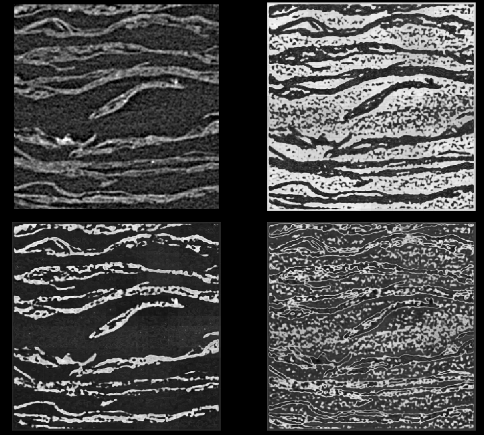
Top left is the raw CT. The other three are what WNet3D makes of it, having never been shown a label. One channel commits hard to sheet-or-not, another keeps the interior texture, a third picks out boundaries. A feature stack the network chose for itself.
Moving it from cells to sheets took a fair bit of CellSeg3D parameter tuning:
- raised the intensity sigma so it stopped chasing CT speckle
- pushed the reconstruction weight up and the n-cuts weight down, shifting it from “cut this into compact objects” towards “preserve this surface”
I had a second motive for chasing this, which was to see whether the network might pick up the ink. I don’t believe it did, and thinking about it more since, its possible it wouldn’t have been possible with this setup. The N-cuts loss clusters voxels by brightness, and carbon ink on carbonised papyrus has little density contrast, which is the whole reason ink detection is hard in the first place. There’s an irony in the tuning too: raising the intensity sigma to stop it chasing CT speckle is probably what killed any chance, since whatever ink signal exists sits down in that same amplitude band. The two things I wanted were pulling against each other. More training wouldn’t have rescued it either, it would just settle the model further into the solution that ignores ink.
The instinct itself seems fine, though. Self-supervised features on raw scroll CT is roughly what the Vesuvius team are doing for ink detection now, with DINO-style embeddings rather than N-cuts.
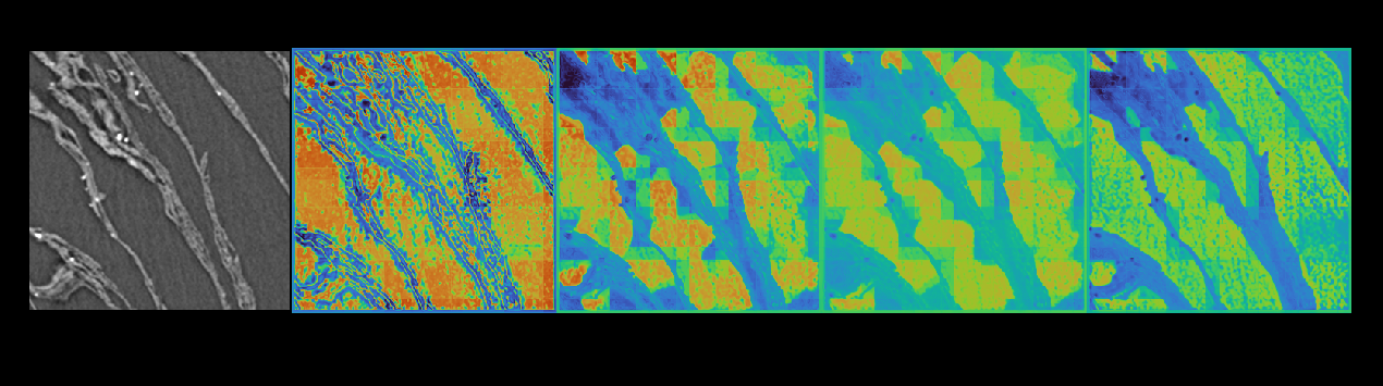
The same slice through several configurations, raw CT on the left. Tuned for cells it breaks the sheets into blobs; tuned for sheets the bands survive as continuous surfaces. Same architecture, same data, no labels. Only the loss weighting changed.
Whether this helped is an important question. One of the submissions I only used nnUNet to train with half of the data using concatenated WNet channels as input and it came within 0.013 of the full-data model. The WNet model had seen all of it anyway and convergence was quicker. Its not too surprising when you think about it as the input is more feature rich!
The whole tech stack:
- ilastik for the first pass, painting labels and getting a feel for the data
- CellSeg3D / WNet3D as the self-supervised preprocessor, a napari plugin
- nnU-Net (ResEncUNet-XL) as the supervised segmenter
- napari for looking at everything in 3D, constantly
- scikit-image and scipy for the postprocessing
- topometrics, the organisers’ official scorer, built under WSL
- vast.ai for GPUs rented by the hour, scaling up as the models got bigger
$$$$ - Dropbox for moving 25 GB of cubes to whichever machine I’d rented
$ - Gemini Pro for writing and debugging Python
$$
All of that software is free and open. The only thing I paid for was compute (my RTX 3080 wasn’t cutting it), and WNet3D pretraining was the slow part at roughly 22 hours for 100 epochs. Inference still had to fit on the two free T4s Kaggle gives you, whatever I trained on. This took some optimizing!
Issues with ground truth
Kaggle competition discussions mentioned discrepancies like holes in the labels, so I profiled all 747 training volumes by topology: separate pieces, enclosed voids, and tunnels through the sheet (inferred from the Euler characteristic, not counted directly). Papyrus doesn’t have holes in it, so any of those is a defect.
137 of the 747 volumes had at least one tunnel, 17 had a void, and the worst had 53 tunnels. That is 707 tunnels and 83 voids sitting inside labels a model will treat as truth.
Cleaning is not the exciting part, i.e., closing to shut the tunnels, hole filling for the voids, dust removal under 500 voxels, and leaving the ignore label untouched so you don’t quietly turn unlabelled regions into background. It closed 576 of the 707 tunnels and all the voids, with 39 volumes rejected by a sanity check. Branch B of my final submission trained on the result.
The organisers realized this and rebuilt the test set mid-competition, which forced a rescore and a two-week extension. They left the training labels alone, since teams had already built pipelines around them.
What I actually submitted
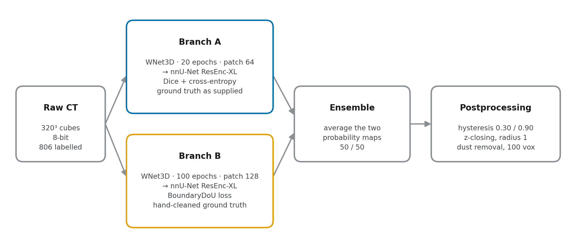
Branch A used the ground truth as supplied. Branch B used my cleaned version, a boundary-aware loss, and a different WNet checkpoint. The diversity between them was worth more than either branch alone.
As far as I can tell, no other team used self-supervised preprocessing. It’s the one genuinely new thing I brought, and it came straight out of working in a different field. The full technical version is in my competition writeup on Kaggle.
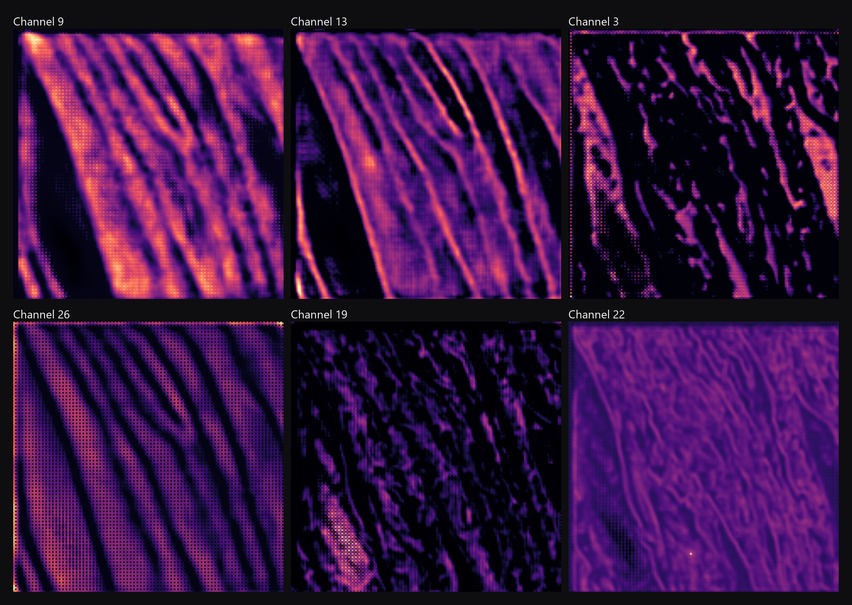
Six of the 32 channels from the last decoder stage of the trained nnU-Net, each scaled on its own, so compare structure rather than brightness. Quite a few of the 32 are dead: the network picked that width from its own dataset fingerprint, not because it needed all of them.
The data itself was 806 labelled cubes from six scrolls, mostly 320³ and 8-bit, of which I had labels for 747. Every label had three values: background, centre surface and ignore. Centre surface was 5% of the voxels. Ignore was 56%, the organisers saying “we’re not confident here, don’t score it” across more than half the annotation. The models trained on it quite happily. It just reiterates how hard annotating data is and its great that nnUNET supports sparse annotated.
The metric shaped every decision
The scoring mattered more than the architecture did, and it wasn’t Dice:
score = 0.35 × surface Dice     boundary alignment, within a tolerance
      + 0.35 × VOI              splits and merges between sheets
      + 0.30 × topological F1   same holes, tunnels and pieces as the truth?
That last term is Betti matching: does your prediction have the same topology as the ground truth, rather than just the same voxels?
On one of my better validation volumes:
surface Dice   0.98      by overlap, essentially finished
topological F1 0.53      by topology, halfway
And 0.53 was near my best. Across my 150 validation volumes the median topological score was 0.16.

I only understood this once I rendered the two volumes side by side. The model found every sheet, in the right place, unsplit and unmerged. What it got wrong was thickness, and running thick is not harmless: bridge two neighbouring surfaces by a voxel here and there and you’ve created handles that were never in the papyrus.
I liked how this metric was designed, and it shows why a single overlap metric is often not enough. If you care about connectivity, whether a neurite is continuous or a vessel is one or many, an overlap metric will tell you everything is fine while your model quietly severs it.
Having a metric at all was the real luxury. Most bioimaging work has no ground truth to score against, often because the structure you’re segmenting is the thing nobody has characterised yet. So the honest answer to “how well did that work?” is that you scrolled through a few fields of view and it looked about right. My 0.53 volume would have passed that test easily.
Things I got wrong
I didn’t get involved in the community as much as I should have. I wasn’t confident about sharing my thoughts and approaches, and joining a team would have been a great way to learn.
My clever postprocessing lost. I ran hyperparameter optimisation over it and reimplemented pieces of the leading teams’ pipelines. A classic case of overfitting. What made my final submission was hysteresis thresholding, a small closing operation and dust removal, close to the simplest thing I tried.
The team that finished 18th did better than me, and after ensembling six models this was their entire postprocessing:
for _ in range(7):
    mask = median_filter(mask, size=3) > 0
Their description: “The post-processing is minimal but very strong.” Two lines of scipy. I use median filters almost every other day and didn’t think to try it.
It wasn’t the architecture
I don’t believe new architectures won this competition. The top solutions ran similar backbones, and the gap between first place and the middle of the field came from postprocessing and ensembling. In one case, seven median filters. None of that is unique to scrolls. It’s how most Kaggle competitions go once a strong default architecture exists. Everyone converges on it, and the winning margin comes from the unglamorous parts either side of it.
Closer to home
I keep coming back to the point that it isn’t always the model. What I liked here was the evaluation, where we had a curated dataset and a carefully designed metric. That meant I could see what was going wrong and where, and that my score and anyone else’s meant the same thing. Without that I’d have looked at the same volumes, decided they were fine, and never known.
Bioimaging mostly hasn’t had this in 3D. In 2D it has, with models like SubCell (Gupta et al., 2025) and benchmarks like CHAMMI (Chen et al., NeurIPS 2023). But large 3D collections are rarely available at pretraining scale, so the work that generalises is on single-cell crops. The self-supervised trick I used as a hack is, at proper scale, roughly what SubCell does for a living (really well!). The scroll competition had all of it:
- a curated 3D benchmark
- an agreed topological metric
- and a few hundred people arguing about it in public. None of that was fast or free of course. It took years of annotation work, a $200k prize pool, and the millions of $$$ funding behind both.
The closest we have is the Cell Tracking Challenge: over a decade of shared 2D+time and 3D+time datasets, and two Nature Methods papers analysing what the field’s methods actually do. It’s why a tracking result means the same thing in two different labs. What it has never had is a few hundred people turning up at once, which is why it was good to see Biohub put cell tracking on Kaggle.
Australian facilities are sitting on the raw material for the 3D version. WEHI’s archive alone is 2 to 3 petabytes of confocal, light-sheet and lattice light-sheet data, and every imaging facility in the country has its own version of the same thing: well acquired, genuinely valuable, and not always AI-ready.
We’ve started on ours. Building foundation models for 3D microscopy is about curating that archive, pretraining and benchmarking on it. In the near term that makes the everyday jobs more tractable on large data: segmentation, tracking and feature extraction from a handful of annotations rather than hundreds. The more open question is whether the embeddings encode any biology of their own. Does a drug, a mutation or a disease that alters cells or tissue architecture separate from a control? And if two of them act the same way, do they land together without anyone deciding in advance what to measure?
One institute’s archive isn’t enough to be a benchmark for a field though. What we don’t have is a 3D benchmark that anyone outside the institute that built it can score against. The question is, what would it take to put one in front of the same crowd that just spent three months arguing about papyrus? If you have a well-annotated 3D dataset, or you’d like to help build one, I’m always up for a chat. Find me on LinkedIN.
Go and try this one
That cell tracking competition ends Sep 2026: light-sheet imaging of zebrafish embryos from the Royer group, tens of thousands of cells to follow through space and time. Their stated goal is transparent, community-driven standards for evaluating cell tracking, which is the same argument pointed at our own data instead of somebody’s scroll.
You don’t need to win. I didn’t, and I learned more in three months of evenings than in about a year of reading papers.
Enter it, publish your notebook and contribute to discussions.
The competition was Vesuvius Challenge: Surface Detection on Kaggle, and my technical writeup is here. The live one as of August 2026 is Biohub: Cell Tracking During Development. The 3D microscopy foundation model project takes students at Honours, Masters and PhD level, and through the Medical Student Research Internship program. Happy to talk to anyone thinking about having a go.